The concept of producer equilibrium in economics is determining at what level a firm maximizes its profit. That occurs when the firm selects the best combination of inputs necessary to attain any output level at the lowest cost, as long as marginal costs equal marginal revenue. Understanding producer equilibrium is very important for students and businesses alike in understanding why firms can optimize their production decisions under competitive and monopolistic markets.
What is Producer Equilibrium?
Producer equilibrium refers to the profit maximization position of a firm when choosing a fair mix of inputs and output. A firm is said to be in an equilibrium position when its cost equals its revenue with no incentive to expand or contract the level of production. A firm is said to be under equilibrium conditions when the marginal cost of producing an additional unit of a product is equal to the marginal revenue earned through the sale of that unit. The relationship would thus provide firms with the ideal quantity of goods that should be produced and sold whereby profits will have been maximized, and any deviation from this point would only serve to decrease the profit in question.
Assumptions of Producer’s Equilibrium
Before delving into how producer equilibrium is reached, it is worthwhile to scrutinize the assumptions that comprise the model. Such assumptions give an economic environment a stylized form and make the analysis more relevant to reality.
- Rational Behavior: It is assumed that the firm behaves rationally, which means it maximizes its profit.
- Perfect Knowledge: The firm has perfect knowledge regarding costs, demand, and prices.
- Constant Technology: The technology employed in the production process does not alter during the period of analysis.
- Perfect Competition: It is assumed that there is perfect competition. The firms are taken as price-takers
- Factor Substitutability: The factors of production are assumed to be substitutable to some extent.
Methods of Determining Producer’s Equilibrium
To determine producer equilibrium, economists generally employ two approaches: the Total Revenue – Total Cost (TR – TC) Approach and the Marginal Revenue – Marginal Cost (MR – MC) Approach.
Total Revenue – Total Cost (TR – TC) Approach
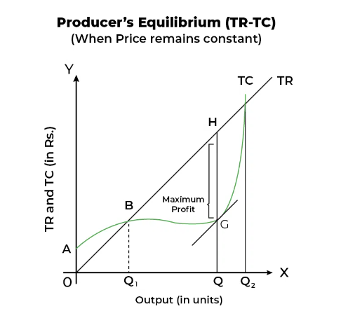
Under this approach, the producer equilibrium is obtained as a point that maximizes the difference between total revenue and total cost. This phenomenon can also be explained by graphing the curves of total revenue and total cost.
- Total Revenue (TR): Total revenue is defined as the amount of revenue earned by a firm when it sells the product. It is expressed as TR = Price x Quantity.
- Total Cost TC: Total cost describes all the costs a firm encounters in the production process, whether fixed or variable.
At the quantity of output where TR is maximum and TC is minimum, profit maximization takes place. Anything more or less quantity of output than that will be bound to result in smaller profits or losses.
| Output | TR | TC | Profit |
|---|---|---|---|
| 1 | 100 | 50 | 50 |
| 2 | 200 | 100 | 100 |
| 3 | 280 | 160 | 120 |
| 4 | 350 | 250 | 100 |
| 5 | 400 | 360 | 40 |
In this table, the profit is maximized at the third unit of output, where the difference between TR and TC is the highest (120).

Marginal Revenue – Marginal Cost (MR – MC) Approach
The MR-MC approach is more often used in economic theory for comparison purposes between MR and MC. MR-MC is a method that compares the marginal revenue along with the marginal cost of producing additional units of output. The term marginal revenue refers to the income received from selling one extra unit, while the term marginal cost refers to the cost incurred by producing one more unit.
- Producer equilibrium is achieved when:
MR = MC
If MR > MC then the firm should expand production. Since it is getting more by selling a unit than the cost incurred to produce it, if MR < MC then the firm should contract by reducing its production so that losses are avoided at least. Equilibrium is thus obtained at the level where MR = MC.
Example:
| Output | MR | MC |
|---|---|---|
| 1 | 100 | 70 |
| 2 | 90 | 80 |
| 3 | 80 | 80 |
| 4 | 70 | 90 |
In this example, the equilibrium is reached at the third unit of output, where MR equals MC (80 = 80).

Isoquant Curves
Isoquants have become particularly important in the analysis of producer equilibrium. An isoquant curve is a graphical representation of all the combinations of two inputs into a given level of output, say labor and capital. These curves indicate the tradeoffs that the firm is willing to accept between two inputs at one level of output.
Isoquants are similar in appearance to indifference curves in consumer theory, except that the former denote not a preference but rather a production possibility. The isoquant map can also help a firm select the appropriate input bundle concerning minimum cost and maximum output.
Characteristics of Isoquants
- Downward Sloping: Isoquants slope downward. That is, the more of one input, the less of another is necessary to produce the same output.
- Convex Shape: Isoquants will reflect the nature of the curve of diminishing marginal returns by turning convex to the origin.
- Non-Intersecting: No two isoquants can intersect because each represents a different level of output.
Isocost Lines
An isocost line represents all combinations of inputs that a firm can purchase given a certain total cost. It is a straight line because the firm faces perfectly competitive input prices. The slope of the isocost line is determined by the ratio of input prices.
Producer equilibrium with isoquants and isocosts. Here an isoquant is said to be the least-cost combination of inputs required to produce a given level of output when it is tangent to an isocost line.
Graphical Example:
The firm achieves equilibrium when the slope of the isoquant (the marginal rate of technical substitution) equals the slope of the isocost line (the ratio of input prices). At this point, the firm cannot reduce costs further without reducing output.
Producer Equilibrium is another related concept in economic theory, taken by firms to find the correct mix of outputs and inputs so that profit maximization can be done. Investigating both the TR-TC approach and the MR-MC approach, and with the help of isoquant curves and isocost lines. The firm will thus be made capable of producing efficiently. Not only theoretical but also highly practical, producer equilibrium is a very serious guide for firms on real-life choices over production. By default, on production choices that can be made in real life.
Producer Equilibrium FAQs
What is the difference between TR-TC and MR-MC approaches in producer equilibrium?
The TR-TC approach focuses on maximizing the difference between total revenue and total cost, while the MR-MC approach finds equilibrium where marginal revenue equals marginal cost.
How do isoquant curves help in producer equilibrium?
Isoquant curves show different combinations of inputs that produce the same output, helping firms choose the least-cost combination of inputs for a given output level.
What is the significance of isocost lines in producer equilibrium?
Isocost lines represent combinations of inputs a firm can afford. Producer equilibrium occurs where an isoquant curve is tangent to an isocost line, minimizing production costs.
What assumptions are made in determining producer equilibrium?
Assumptions include rational behavior, perfect competition, constant technology, and the ability to substitute inputs.
What is the optimal point of production for a firm?
The optimal point is when the firm maximizes profit by ensuring marginal cost equals marginal revenue, and it produces at the lowest cost for the desired output level.


